Io, ChatGPT e Lorenza

Secca come una fucilata: "Ma tu non hai paura che ChatGPT ti rubi il posto di lavoro?"

Sento una lievissima fitta agli addominali, è colpa evidentemente della panca bassa che abbiamo fatto stamattina a yoga, ma significa anche che la domanda mi ha fatto contrarre i muscoli. Giunge quasi alla fine di una conversazione interessante su ChatGPT, su come può cambiare lo scenario del lavoro, sui mestieri che si estingueranno e sulle professionalità che resteranno in sella a questo cavallo imbizzarrito e artificiale di cui tutto parlano. Respiro un attimo, ci penso su, un altro respiro e poi: "Lorenza, no, non credo che ci rimetterò il posto..." ChatGPT non è preciso, lo hanno beccato a contraddirsi molte volte, ma questo è tipico del linguaggio naturale, di come comunicano gli umani, tutto un ripetere cose lievemente diverse, infarcendo di contesto, di cose implicite e incerte, dando per scontato che l'interlocutore capisca e riempia i buchi del discorso. È ovvio, se ci pensate, che sui dettagli ci contraddiciamo spesso, non fosse altro perché tagliamo corto e non ripetiamo tutto quello che, forse, logicamente dovremmo. Tiriamo via dritto, e le scorciatoie possono tralasciare i dettagli, sono fatte apposta. La maggior parte delle nostre imprecisioni non è grave, aiuta la sintesi e nessuno te le rinfaccia (certo, ci sono anche i rompicoglioni...). I politici sono casi esemplari: cambiano idea sin verguenza come banderuole, dicono anche fesserie monumentali e poi si scusano, a base di "non mi avete capito", "non prendetemi alla lettera", "avete estrapolato dal contesto" (appunto, è semplre colpa del contesto!) e, per farla breve, li votiamo sempre nonostante le imprecisioni. "Ma io sono un matematico e la mia materia è una delle poche, pochissime, in cui la precisione estrema è l'essenza e la bellezza delle cose, non un'appendice cosmetica". E continuo dicendo che non ho paura di ChatGPT nemmeno nel mio secondo lavoro, quello di insegnante: "Non mi può sostituire perché educare significa tirare fuori dagli studenti quello che sono, serve capacità di coinvolgerli, di motivarli, di accendere un fuoco. Non si tratta solo di passare contenuti, ci vuole sempre un supplemento d'anima". ChatGPT non fa nulla di tutto questo, è uno zero nei confronti di un professore che ha letteralmente il potere di cambiarti la vita (se è bravo, d'accordo; ci sono anche quelli che ti fan venire il latte alle ginocchia!)

Eppure, la domanda m'inquieta. Lorenza scrive su un giornale locale, nella sua voce serpeggia curiosità, ammette di essere felice perché può scrivere di quel che le interessa (cosa rara, wow!) Fa le domande giuste, non cerca risposte semplici, memorizza la mia difficoltà a darle visioni e previsioni su quel che sarà, sorride all'altro lato della cornetta quando sparo che secondo me in 5 anni ChatGPT potrebbe avere già sostituito tutta una serie di lavoratori impegnati in mansioni intellettuali a bassa intensità, dato che altri intervistati le hanno detto che serviranno 10 o trent'anni.

La nostra bella conversazione finisce ma io continuo a mulinare cattivi pensieri: "ChatGPT, che diamine vuoi da me e dai miei studenti?", mi chiedo.  Decido di prendere un problema da compito, un esercizio standard per i miei studenti di "Computational tools", e di darlo in pasto all'AI: risolvi l'equazione x^3+x+1=0. A suo modo, non è un problema difficile, "x alla terza più x più uno uguale a 0", ma non c'è una formula risolutiva semplice come per le equazioni di secondo grado, quella che a un certo punto della vita abbiamo imparato tutti (sorvolo sul fatto che quanto ho scritto è un'imprecisione... Cardano abbi pietà ma non finirei più!)

Ogni computer dovrebbere risolvere quell'equazione di terzo grado "facilmente" e produrre il risultato. Vuoi vedere che da ora in poi i miei studenti mi possono fregare e trovare quel numero semplicemente chiedendo a ChatGPT?

solve the problem x^3+x+1=0

ChatGPT: Unfortunately, the equation x^3 + x + 1 = 0 does not have an algebraic solution that can be expressed in terms of elementary functions. This is because the equation is a cubic equation, and there is no general formula for solving cubic equations algebraically like there is for quadratic equations.

However, the equation can be solved numerically using numerical methods, such as the Newton-Raphson method or the bisection method. These methods involve iteratively refining an initial guess for the solution until it converges to the true solution.

Formulo il problema: risolvi un'equazione di terzo grado (8 maggio 2023)

È una bella filippica, fin qui tutto ok, ma non c'è ancora traccia della soluzione. Del numero, intendo.

Using the Newton-Raphson method, ... the solution to the equation x^3 + x + 1 = 0 is approximately -1.324717957244746.

Resto senza fiato! Sto gran figlio (o figlia?) dell'intelligenza artificiale e di un computer ha trovato la soluzione! E così potranno fare i miei studenti, senza studiare un solo minuto. Sono destinato alla disoccupazione, preparate anche per me il nuovo reddito di cittadinanza!

Non mi resta che dirmi "finché c'è vita c'è speranza" ma decido, per puro scrupolo, di controllare. Scrivo due righe in R, un altro programma di cui mi fido da decenni:

> f <- function(x) x^3+x+1

> uniroot(f,c(-2,0)) # trova la soluzione compresa fra -2 e 0

$root [1] -0.6823219

Vedo che la soluzione è -0.682. (sto arrontondando per risparmiarvi file di cifre). Ma ChatGPT aveva detto -1.325 e rotti... Un ghigno si scolpisce sulla mia faccia dato che ChatGPT, con grande faccia tosta, ha dato la soluzione sbagliata! Provo ad aiutarlo, se -1.325 fosse la soluzione dovrei ottenere che f(-1.325)=0.

compute f(x) with x= -1.324717957244746

ChatGPT: To compute f(x) with x = -1.324717957244746, we substitute this value of x into the function f(x) = x^3 + x + 1:

f(-1.324717957244746) = (-1.324717957244746)^3 + (-1.324717957244746) + 1

= -1.324717957244746

Therefore, f(-1.324717957244746) = -1.324717957244746.

Un altro pezzo di sessione (8 maggio 2023)

Ora, fidatevi, il ragionamento è giusto ma i conti sono tutti sbagliati e f(-1.324717957244746)=-2.649436. Riassumendo per i comuni mortali: ChatGPT sbaglia a trovare la soluzione e sbaglia pure a controllare se ha fatto giusto! Se fosse uno studente non se la passerebbe bene a questo punto. Provo a insistere, uso perfino un filo d'ironiaa, magari torna in sé:

that's strange as i got f(-1.324717957244746) = -2.649436

ChatGPT: I apologize for my mistake. You are correct.

To compute f(x) with x = -1.324717957244746, we substitute this value of x into the function f(x) = x^3 + x + 1:

f(-1.324717957244746) = (-1.324717957244746)^3 + (-1.324717957244746) + 1

= -2.64943585095

Ci sono segni di ravvedimento: intanto si scusa, come un Salvini qualsiasi dopo che ha detto una vaccata, vabbuò! Poi fa il conto giusto (ma il risultato gliel'avevo già detto io formulando la domanda), sempre meglio di nulla. Penso che forse ce la può fare e riattacco:

but you told me that f(-1.324717957244746)=0. can you try to solve the equation correctly?

ChatGPT si scusa un'altra volta e scrive questo sproloquio:

I apologize for the confusion and my previous incorrect answer. Here's an attempt to solve the equation x^3 + x + 1 = 0 using Cardano's method, which is a standard method for solving cubic equations:

First, we express the equation in the form x^3 = -x - 1:

x^3 = -(x + 1)

Next, we introduce a new variable y such that x = z - b/3, where b is the coefficient of the quadratic term, which is 0 in this case. This gives:

(z - b/3)^3 = -(z - b/3 + 1)

Expanding the left-hand side and simplifying, we get:

z^3 - 3bz^2/9 + 3b^2z/27 - b^3/27 = -z + 1/3

Multiplying both sides by 27 and simplifying, we obtain:

27z^3 - 27z + 9b^2z - b^3 + 3 = 0

Substituting b = 0, we get:

27z^3 - 27z + 3 = 0

Dividing both sides by 3, we obtain:

9z^3 - 9z + 1 = 0

Now, we need to find a root of this equation, which can be done using numerical methods such as the Newton-Raphson method. A root of this equation is approximately z = 0.4533976515.

Finally, we can obtain the three solutions of the original equation x^3 + x + 1 = 0 by using the formula x = z - b/3:

x1 = z - b/3 = 0.4533976515 - 0/3 = 0.4533976515 x2 = αz - β/3 = -1.088186771 - 0.5i x3 = αz - β/3 = -1.088186771 + 0.5i

where α = (-1 + sqrt(-3))/2 and β = (1 - sqrt(-3))/2 are the complex cube roots of unity.

Il punto è che  il valore z=0.4533976515 menzionato da ChatGTP, nuovamente, non è una soluzione! ChatGPT ci ha provato, e ha scritto una rampegada che contiene polvere di verità anche se, per notarlo, devi essere un matematico. Insomma, non è uno studente brillante ma ci ha provato, sbrodolando sia cose corrette che errori. Forse "ragiona" e prende dai siti alcune informazioni giuste ma poi o non le capisce o le usa male e, invitabilmente, produce il risultato sbagliato, questo povero z=0.453 che non c'entra con il numero giusto -0.682 (che R aveva trovato subito).

È ora di concludere: i miei studenti dovranno studiare ancora un po' o imparare altri trucchi dato che non si possono fidare di ChatGPT, che le spara grosse a raffica. Per ora nessuno mi ruberà la cattedra. Già, per ora: i sistemi di AI apprendono, si esercitano, a loro modo imparano dagli errori e forse proprio io, che pure l'ho preso per il culo, gli sto insegnando a risolvere le equazioni di terzo grado come si deve. E non è detto che, fra qualche settimana o mese, non riesca a darmi la risposta giusta con disinvoltura. Insomma, lo terrò sotto osservazione.

Continuo a pensare che su altri fronti ChatGPT sia ancora più indietro: forse un buon docente riesce a incuriosire gli studenti, forse gli fa capire a cosa serve quell'equazione, forse presenta esempi illuminanti e legati al rendimento dei BTP, forse qualcuno inizia a percorrere gli impervi sentieri della matematica computazionale e della programmazione proprio grazie alle lezioni. Forse. Ma temo serva umiltà anche qui e non è detto che fra un po' ChatGPT non riesca ad essere simpatico e travolgente più di me e dei miei colleghi!

ps. In realtà il post non è finito e domani aggiungerò "Io, ChatGPT e julia" perché questo esperimento mi ha dato una frustata e ho deciso che, in barba al fatto che sto invecchiando, insegnerò anche un altro di linguaggio di programmazione oltre a R. Non voglio inseguire ChatGPT, è lui che deve rincorrere me!

ps2. Vi voglio anche raccontare un paio di altre cose "sbagliate" e di come ChatGPT si vada usato con cautela, le cantonate sono sempre in vista!   

Complex coloring and contour levels

I was recently fascinated by the illustration taken from the leaflet https://www.maa.org/sites/default/files/pdf/Mathhorizons/pdfs/ColoringPage_MH_Nov17.pdf

I knew that complex functions could be colored in mesmerizing ways but the little book by Julie Barnes, William Kreahling, and Beth Schaubroeck, “Coloring book of complex function repesentation”, MAA Press, 2017, explores new avenues and, say, I never realized that contour lines could be used to obtain beautiful images. Moreover, I teach students how to draw contour curves of two dimensional functions like \(f(x,y)\) and thought this could be a funny example (though, it is really another story when you tweak functions of the complex plane in itself.) Hence, I bought the book (actually, I got it out of the bonus points awarded by writing reviews on Mathscinet) and decided to give R a try. Take the function \[ f(x)=z^2-\frac{0.6}z, \] where \(z\in\mathbb{C}\) and consider 6 nested applications of the function with itself \[ f^6(z)=f(f(f(f(f(f(z)))))):=f6(z). \] (don’t ask me how the authors found that, the book provides plenty of insights and I do not want to spoil all the fun!) Of course, \(f6(z)\) is a complex number and we are going to plot the \(z\)’s such that the real part of \(f6(z)\) is null. In other words, we plot the zero-contour level of \(\Re (f6)\) on the rectangle \([-0.85,1.35\times [-1.4,1.4]\) of the complex plane. If you prefer, we want to find the complex points that are mapped to the imaginary axis after 6 applications of \(f\). The standard (so to say!) way to plot contour lines in is to use outer and contour. This time, I’m not plotting \(f(x,y)\) where \(x,y\) are two real numbers but I’ll compute \(f6(x+i\ y)\), where \(z=x+i\ y\):

fz <- function(z) z^2-0.6/z
fz6 <-function(z) fz(fz(fz(fz(fz(fz(z))))))
f6 <- function(x,y) fz6(x+1i*y)
x <- seq(-0.85,1.35,len=1001)
y <- seq(-1.4,1.4,len=1001)
m <- outer(x,y,f6) # this is a matrix of complex numbers
contour(x,y,Re(m),levels=c(0),drawlabels=F,axes=F) 
# Re(m) takes the real parts

I was pretty much happy of the work: a few lines of code fill the matrix \(m\) with all the complex values of \(f6\) for all \(x+i\ y\) (\(x\) and \(y\) are taken from the sequences). Then, a contour on the real part of the matrix is displaying this marvel, if you share my enthusiasm… I decided to tamper a bit with the filling of the contours using colors and, in so doing, showing how to extract the points contained in all in all the (possibly many) components of contour lines:

cl <- contourLines(x,y,Re(m),levels=0)
pal <- topo.colors(48)
contour(x,y,Re(m),levels=c(0),drawlabels=F,axes=F)
for(i in 1:length(cl)) polygon(cl[[i]]$x,cl[[i]]$y,col=pal[i %% 12+1])

The variable cl is a list with the points of all the components of the zero-level contours and pal is a palette of colors (you can unleash your imagination and change palette). Then a for loop fills with different shades every single contour in I decided to use this and other variations to send Christmas cards to friends and relatives. I love math and (also) wrote the complex function \(f(z)\) on the card but really felt the pictures were nice and needed no complexity (!) at all to be enjoyed. The picture that originates all the story is related to another complex function and displays three contours at one time. Easy as a piece of cake:

fz <- function(z) z^3+(-0.2+0.11*1i)/z^3
fz3 <-function(z) fz(fz(fz(z)))
f3 <- function(x,y) fz3(x+1i*y)
x <- seq(-1.08,1.08,len=1001)
y <- seq(-1.3,1.3,len=1001)
m <- outer(x,y,f3) # this is a matrix of complex numbers
contour(x,y,Re(m),levels=c(-2,0,2),drawlabels=F,axes=F) 
# Re(m) takes the real parts

Have a colorful (and not that complex) new yeaR!

Chaos, bifurcation diagrams and Lyapunov exponents with R (2)

(The first part of this article can be read here)

Iteration of one-dimensional maps can generate stunning complexity and famed examples of chaotic behavior.  R can be used to get the flavor of this richness and reproduce some of the most famous pictures in the history of science, such as the bifurcation diagram of the logistic map or the representation of its Lyapunov exponents.

Given a one dimensional map depending on a parameter, a bifurcation diagram shows the stable structures (fixed point, cycles, attractors) visited by the dynamics for each value of the so called "bifurcation parameter".  Resisting the temptation to use again and again the beloved logistic map, consider instead the following dynamical system

x(t+1)=a cos x(t),  

taken from exercise 10.2.6, page 389 of Strogatz, "Nonlinear Dynamics and Chaos: With Applications to Physics, Biology, Chemistry, and Engineering".  The following script defines a function to get the bifurcation diagram for a given map (I modified some existing code, but I was not able to find and credit the exact source: https://web.stanford.edu/group/heeh/cgi-bin/web/node/59, say, has the same ideas. I defined a function and removed the use of "expression" and "evalf").  See also the post at https://www.r-bloggers.com/dynamical-systems-mapping-chaos-with-r/

bif_diagram <- function(f=function(x,a) (a*x*(1-x)),alow=2.5,ahigh=4,
                        thinness=1000, transient=200, collect=200){
        # f function, parameter must be named a
    n <- 1
    R <- seq(alow,ahigh,length=thinness)
    data <- matrix(0,collect,thinness+1)

    for(a in R){
      x <- runif(1) # random initial condition
      ## first converge to attractor
      for(i in 1:transient){
        x <- f(x,a)
      } # collect points on attractor
      for(i in 1:collect){
        x <- f(x,a)
        data[i,n] <- x
      }
  n <- n+1
}

data <- data[,1:thinness]
yrange <- range(data)+c(-0.1,0.1)
plot(R,data[1,], pch=".", xlab="a", ylab="States",ylim=yrange)
for(i in 2:collect) points(R,data[i,],pch=".")
}

Now, enter

f <- function(x,a) a* cos(x)
bif_diagram(f,alow=0.5,ahigh=4)

Bifurcation diagram for f(x,a)=a cos x, when a is the range [0.5,4].

You can see that, for low values of the parameter a, there are unique fixed points or simple cycles.  Then, through  a series of (quite typical) period-doubling bifurcations, chaos appears and suddenly disappears when the parameter crosses 3.  bif_diagram has defaults parameters that can be adjusted to specify the parameter's interval of interest or increase/decrease the resolution and legibility of the resulting plot.

One of the most interesting signature of chaos is the divergence of orbits arbitrarily close in their initial conditions.  Broadly speaking, orbits are stretched apart by some systems and a positive stretching rate is signaling the presence of chaos.  The Lyapunov Exponents (LE) is the average (exponential) growth rate of the divergence of initially nearby orbits.  LEs can be computed, for any value of the bifurcation parameter using the lyap function below, where is assumed that you have properly defined the dynamics f in advance.

lyap <- function(a,trans=300,num=1000){
    x0 <- runif(1)
    for(time in 1:trans){
        x1 <- f(x0,a=a);x0 <- x1
    }
    sl <- 0
    for(time in 1:num){
        x1 <- f(x0,a=a);x0 <- x1
        sl <- sl+log(abs(grad(f,x1,a=a)))
    }
    sl/num
}

In order to graph LEs define a sequence of values of the parameters, use sapply to get the sequence of corresponding exponents by applying lyap to the elements of the sequence and finally plot.  With the same map given above:

a <- seq(0.5,4,length=100)
ly <- sapply(a,lyap)
plot(a,ly,t="l")

Lyapunov exponents for f(x,a)=a cos x, when a is the range [0.5,4].

It can be seen, say, that when a=2, the LE is positive and chaos is in action [Check the bifurcation diagram to get the same intuition for that value of a].  Entering lyap(2) would indeed produce 0.15 (approximately).  In rough terms, this means that divergence of close initial points will be on average amplified by about 15% per iteration of the map over its domain.

To conclude:

• it is fun to try the same things with a slightly modified map: x(t+1)=cos(a x(t)) (the parameter is "inside" the cos);
• if you want to replicate two of the most well-known pictures related to the logistic map, type

  f <- function(x,a) a*x*(1-x)
  bif_diagram(f,0,4)
  

• the graph of LE, seen on page 369 of Strogatz's book is readily obtained through

a <- seq(3,4,len=100)
f <- function(x,a) a*x*(1-x)
ly <- sapply(a,lyap,num=2000)
plot(a,ly,t="l",ylim=c(-1,1));abline(h=0)

Lyapunov exponens for the logistic map, when a is the range [3,4].

Non-linear dynamics and chaos using R (1)

I have been teaching the course "Mathematics" for the PhD students at Ca' Foscari University for a few years. In the lectures I cover some "scattered" material that may prove useful, sooner or later, to develop quantitative models in Economics. One of the weeks of the course is devoted to non-linear dynamics, one-dimensional maps and chaos.
R can be extremely useful to explore the dynamics, compute fixed points or cycles and have a numerical look at the map. The mix of computational techniques and theoretical investigation is widely acknowledged to be fruitful. As Strogatz, "Nonlinear Dynamics and Chaos: With Applications to Physics, Biology, Chemistry, and Engineering", puts it:

The study of maps is still in its infancy, but exciting progress has been made in the last twenty year, thanks to the growing availability of calculators, then computers, and now computer graphics. Maps are easy and fast to simulate on digital computers where time is inherently discrete. Such computer experiments have revealed a number of unexpected and beautiful patterns…

Given a non-linear map \(f\) you may want to plot the time series of states \(x_{t+1}=f(x_t)\), depict the cobweb diagram and look at fixed points, to begin with. Let \(f\) be the immortal logistic map depending on the parameter \(r\).

f <- function(x,r) r*x*(1-x)
bounce <- function(f,init=4,n=10,cobweb=T,timeseries=F,dom=NULL,...){
iterates <- NULL
x0 <- init
for(t in 1:n){
  x1<- f(x0,...)
  iterates[t] <- x1
  x0 <- x1
  }

if(cobweb & !timeseries){
    if(is.null(dom)){
    a <- range(c(init,iterates))[1]-0.5
    b <- range(c(init,iterates))[2]+0.5} else
    {a <- dom[1];b <- dom[2]}
    curve(f(x,...),a,b);grid(col=1);abline(0,1,lty=2)
    lines(c(init,iterates), f(c(init,iterates),...),t="s")
    points(c(init,iterates), f(c(init,iterates),...))
}

if(timeseries){
    plot(0:n,c(init,iterates),t="l")
}

}
bounce(f,0.1,r=3.7,n=100)

bounce computes \(n\) iterates of the map starting from init an plots a cobweb diagram. Defaults may or may not work for a specific map but the plotting domain can be provided if the educated guess doesn't work (here, say, bounce(f,0.1,r=3.7,n=100,dom=c(0,1) would be probably better).

bounce(f,0.1,r=3.7,n=100)

The function bounce shows the 45-degrees line (dashed) and its intersections with the graph of the function: fixed points and their stability can be visually investigated (or found with uniroot). Indeed, the name comes from the repeated "bounces" on the line and on the graph. Setting timeseries=T displays the sequence of states of the dynamics (i.e., the time series) as shown below for \(r=3.8282\), a value that generates intermittency, see page 363 of Strogatz:

bounce(f,0.1,r=3.8282,n=100,timeseries=T)

In a coming post, we'll use R to draw bifurcation diagrams and Lyapunov exponents.

MOOC "Take lineaR decisions" (Ca' Foscari University)

The MOOC "Take lineaR decisions" will begin on September 19th 2016, covering some models of decision making mainly based on computational linear algebra (linear systems and eigenvalues/vectors). The course, delivered by prof. Paolo Pellizzari, can be used to acquire practical skills in the use of the open software R in dealing with matrices, vectors and related optimization problems. In some detail, the 6 online weeks will cover:

1. Famous theorems to solve linear systems
2. Inverses and pseudo-inverses
3. The State Preference Model, replication and arbitrage
4. Optimization (basic and more advanced topics)
5. Eigenvalues and eigenvectors - Introduction to AHP (Analytic Hierarchic Process)
6. Decisions with AHP

The course is aimed at students in economics, sciences, IT and engineering but is also directed to  professionals and to the general public (with adequate analytic skills) interested in formal decision-making, linear algebra, R use and computational tools. A class of students of Ca’ Foscari will work on the material to gain partial credits for their academic program (with additional studying activities).

 

Quizzes at the end of each learning unit are made public in advance and the test can be attempted only once (after the material has been studied. The course "Introduction to Complexity" by Melanie Mitchell used the same clever assessment format). A certificate will be issued to anyone with an average score of 70% or more (on the 6 tests). 

More information and free enrollment at the Open Knowledge platform of Ca' Foscari University (the final questions can be downloaded here).

Nonlinear constraints with a modified constrOptim

I often use constrOptim to quickly solve nonlinear optimization problems. constrOptim works well as a general tool to tackle constrained problems like
\[
\min_{Ax -b \geq0} f(x)
\] 
There are many other options and packages for specific problems but constrOptim is likely to be the first choice when little is known on the problem at hand or for exploratory/quick-and-dirty analysis.

The main problem I have with it is the nature of the constraints: they must be linear (written in matrix form as \(Ax-b≥ 0\)). Often I would like to compute (local) solutions of more general problems of the form
\[
\min_{g(x) -b \geq0} f(x)
\] 
where g(x) takes vector values, one component for each scalar constraint, and is in general nonlinear, i.e., \(g(x)\) cannot be written as \(Ax\).

Hence, I tweaked the code of constrOptim replacing all the occurrences of the linear constraints with my "new" non linear constraints. (In order to do that, I had to discard the chance to use "BFGS" as a solving method, for now...)  The result is a function, called constrOptimNL, see the code below, which can handle non linear constraints if a vector function g(x) and b are provided. All the drawbacks of the old function are inherited, that's life, but now non linear problems can be solved as shown by the following simple but non entirely trivial example in two dimensions.

 f <- function(x,y) x^2*y+x-x*y  
 fb <- function(x) f(x[1],x[2]) #vectorial version of f  
 x <- seq(0,3,length=31)  
 y <- seq(0,3,length=31)  
 z <- outer(x,y,f)  
 #draws a graph  
 image(x,y,z);contour(x,y,z,add=T)  
 polygon(c(0,0,3),c(0,3,0),col="white",density=20)  

Heatmap and contour lines of the objective function, the feasible domain is filled in white.

Consider the constraints \(x\geq0,y\geq 1, x+y\leq 3\), the feasible domain is a triangle with vertices (0,0), (0,3), (3,0): due to linearity, the problem can be solved with

 A <- matrix(c(1,0,-1,0,1,-1),3,2)  
 b <- c(0,1,-3)  
 res <- constrOptim(c(0.5,1.5),fb,NULL,A,b)  
 res

$par
[1] 0.2792393 2.7207607
$value
[1] -0.2683538
$counts
function gradient
246 NA 

...

The same problems can be solved with constrOptimNL, which trivially can handle linear constraints as well:

 g <- function(x,y) c(x,y,-x-y)  
 gb <- function(x) g(x[1],x[2])  
 source("constrOptimNL.R")  
 resNL <- constrOptimNL(c(0.5,1.5),fb,NULL,gb,b)  
 resNL

$par
[1] 0.2792393 2.7207607
$value
[1] -0.2683538
$counts
function gradient
246 NA

... 

Assume now that some non linear constraint is involved in the optimization problem: \(x\geq0,y\geq1,(x-1)^2+(y-1)^2\leq1\), the feasible domain is now the upper half-circle centered at (1,1) with unit radius. This problem has nonlinearities in the constraints and cannot be solved with the standard constrOptim.

 g <- function(x,y) c(x,y,-(x-1)^2-(y-1)^2)  
 b <- c(0,1,-1)  
 resNL <- constrOptimNL(c(0.5,1.5),fb,NULL,gb,b)  
 resNL$par  

[1] 0.2649931 1.6780596 

A graph shows that this is indeed the correct solution:

 alpha <- seq(0,pi,len=31)  
 image(x,y,z); contour(x,y,z,add=T)  
 polygon(cos(alpha)+1,sin(alpha)+1,col="white",density=20) #draws the half-circle  
 points(resNL$par[1],resNL$par[2])  

Contour levels and a nonlinear feasible domain in white (the solution is plotted with a filled circle).

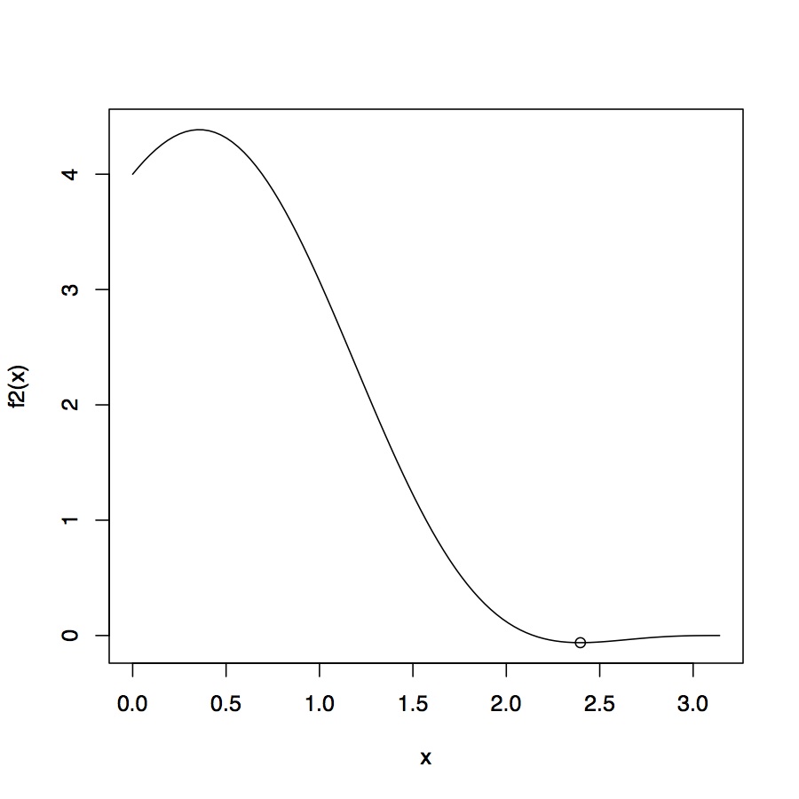
You can check the solution more formally substituting the nonlinear constraint in polar coordinates, \(x=\cos\alpha+1,y=\sin\alpha+1\):

 f2 <- function(alpha) f(cos(alpha)+1,sin(alpha)+1)  
 curve(f2,0,pi)  
 sol <- optimize(f2,c(0,3))  
 points(sol$minimum,sol$objective)  
 c(cos(sol$minimum)+1,sin(sol$minimum)+1)  
 #"same" as resNL  

Objective function restricted to the half-circle

The code

The code for constrOptimNL is given below (in this version the parameter grad is kept for compatibility with constrOptim but will never be used: Nelder-Mead and SANN are derivatives free and invoking BFGS stops the function). Hope this helps.

 constrOptimNL <- function (theta, f, grad, g, ci, mu = 1e-04, control = list(),   
   method = if (is.null(grad)) "Nelder-Mead" else "BFGS", outer.iterations = 100,   
   outer.eps = 1e-05, ..., hessian = FALSE)   
 {  
   if(method=="BFGS") stop("method BFGS not available, use Nelder-Mead or SANN")  
   if(!is.null(control$fnscale) && control$fnscale < 0)   
     mu <- -mu  
   R <- function(theta, theta.old, ...) {  
     ui.theta <- g(theta,...)  
     gi <- ui.theta - ci  
     if (any(gi < 0))   
       return(NaN)  
     gi.old <- g(theta.old,...) - ci  
     bar <- sum(gi.old * log(gi) - ui.theta)  
     if (!is.finite(bar))   
       bar <- -Inf  
     f(theta, ...) - mu * bar  
   }  
   dR <- function(theta, theta.old, ...) {  
     ui.theta <- g(theta,...)  
     gi <- drop(ui.theta - ci)  
     gi.old <- drop(g(theta.old,...) - ci)  
     dbar <- colSums(ui * gi.old/gi - ui)  
     grad(theta, ...) - mu * dbar  
   }  
   if (any(g(theta,...) - ci <= 0))   
     stop("initial value is not in the interior of the feasible region")  
   obj <- f(theta, ...)  
   r <- R(theta, theta, ...)  
   fun <- function(theta, ...) R(theta, theta.old, ...)  
   gradient <- if (method == "SANN") {  
     if (missing(grad))   
       NULL  
     else grad  
   }  
   else function(theta,...) dR(theta, theta.old, ...)  
   totCounts <- 0  
   s.mu <- sign(mu)  
   for (i in seq_len(outer.iterations)) {  
     obj.old <- obj  
     r.old <- r  
     theta.old <- theta  
     a <- optim(theta.old, fun, gradient, control = control,   
       method = method, hessian = hessian, ...)  
     r <- a$value  
     if (is.finite(r) && is.finite(r.old) && abs(r - r.old) <   
       (0.001 + abs(r)) * outer.eps)   
       break  
     theta <- a$par  
     totCounts <- totCounts + a$counts  
     obj <- f(theta, ...)  
     if (s.mu * obj > s.mu * obj.old)   
       break  
   }  
   if (i == outer.iterations) {  
     a$convergence <- 7  
     a$message <- gettext("Barrier algorithm ran out of iterations and did not converge")  
   }  
   if (mu > 0 && obj > obj.old) {  
     a$convergence <- 11  
     a$message <- gettextf("Objective function increased at outer iteration %d",   
       i)  
   }  
   if (mu < 0 && obj < obj.old) {  
     a$convergence <- 11  
     a$message <- gettextf("Objective function decreased at outer iteration %d",   
       i)  
   }  
   a$outer.iterations <- i  
   a$counts <- totCounts  
   a$barrier.value <- a$value  
   a$value <- f(a$par, ...)  
   a$barrier.value <- a$barrier.value - a$value  
   a  
 }